# Objectives 目标

• Understand Uniform Distribution and Normal Distribution
  了解均匀分布和正态分布
• Know how to generate the uniform and normal random numbers
  知道如何生成均匀和正态随机数
• Know how to use q- function to find the quantiles of the normal distribution
  知道如何使用 q- 函数找到正态分布的分位数

# Uniform Distribution 均匀分布

Uniform Random Variable 均匀随机变量

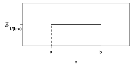
A uniform random variable is a continuous random variable for which every outcome in an interval is equally likely.
均匀随机变量是一个连续的随机变量，在一个区间内，每个结果的可能性都相等。

• Example: $X$ is a random real number taken from $[0,1]$.
  $X$ 是一个随机实数取自 $[0,1]$ 。

• We can use runif(n) to generate random number taken from $[0,1]$.
  我们可以 runif(n) 用来生成随机数取自 $[0,1]$ 。

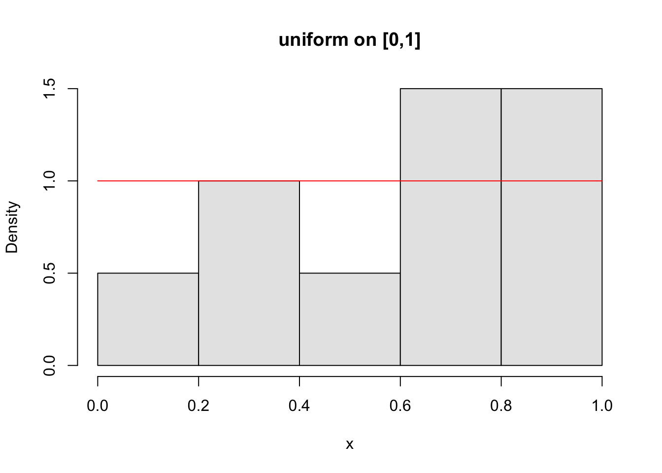
n <- 10 # number of sample size

x <- runif(n) # generate random numbers taken from the interval [0,1]

hist(x,probability=TRUE,col=gray(.9),main="uniform on [0,1]")

curve(dunif(x,0,1),add=T,col = "red")

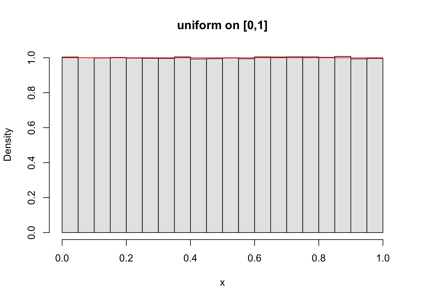
What will happen if increasing the number of the sample size?
如果增加样本数量会发生什么？

n <- 1e6 # number of sample size

x <- runif(n) # generate random numbers taken from the interval [0,1]

hist(x,probability=TRUE,col=gray(.9),main="uniform on [0,1]")

curve(dunif(x,0,1),add=T,col = "red")

• Notation: $X\sim U[a,b]$

• Probability Density Function pdf :
  $f(x) = \frac{1}{b-a}$ for $a\leq x\leq b$

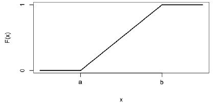
• Cumulative Distribution Function cdf :
  For $a\leq x\leq b$

  $$F(x)= P(a \leq X \le x) = \int_a^x f(t)d t=\int_a^x \frac{1}{b-a}d t=\frac{x-a}{b-a}.$$

• Expectation & Variance 期望值与方差

$$\mu = E(X) =\int_a^b x\frac{1}{b-a} d x=\left.\frac{x^2}{2(b-a)}\right|_{a}^b=\frac{a+b}{2}$$

$$\sigma^2 = var(X) = E(X^2)-[E(X)]^2 = \int_a^b x^2\frac{1}{b-a} d x - \left(\frac{a+b}{2}\right)^2= \left.\frac{x^3}{3(b-a)}\right|_{a}^b-\frac{(a+b)^2}{4} = \frac{(b-a)^2}{12}$$

# Important R functions

• To generate random numbers, pdf (aka pmf), cdf, and quantiles.
  生成随机数、pdf（又名 pmf）、cdf 和分位数。

• The prefixes for these functions are:
  这些函数的前缀是：

# Example 1

Suppose $X \sim U[-1,1]$

n <- 1e6 # number of sample size

x <- runif(n,-1,1) # generate random numbers taken from the interval [-1,1]

hist(x,probability=TRUE,col=gray(.9),main="uniform on [-1,1]") # histogram of the relative frequency - probability=TRUE

curve(dunif(x,-1,1),add=T,col = "red") #plot the probability density function of X

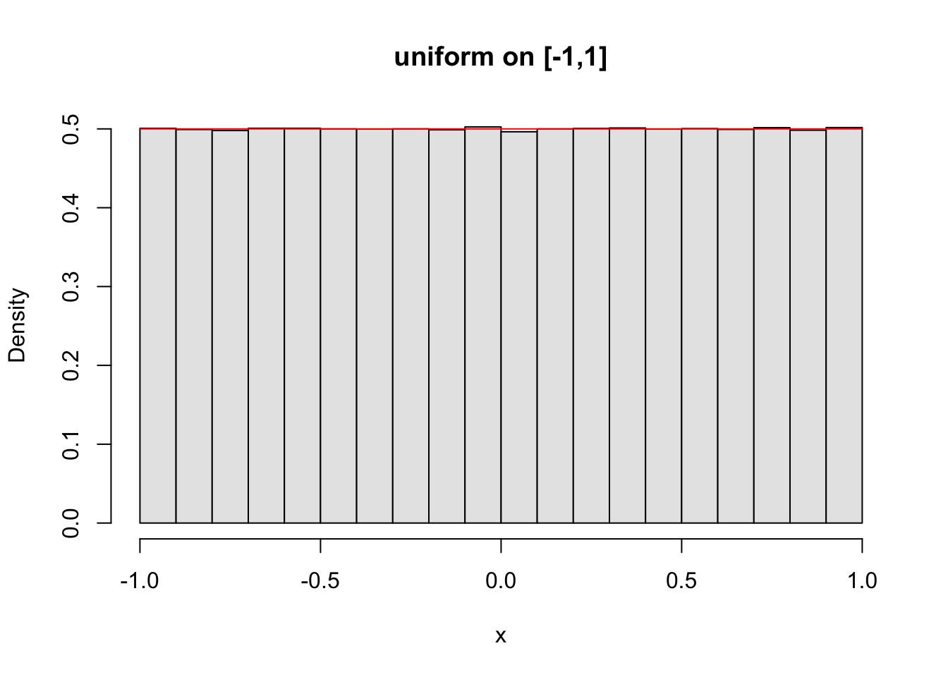
punif(0.5, min =-1, max = 1) # find the P(-1 <= X <= 0.5)

[1] 0.75

qunif(0.5, min = -1, max = 1) # find the median of X

[1] 0

mean(x) # find the sample mean

[1] 0.0002108174

var(x) # find the sample variance

[1] 0.3333544

# In-class Exercise: Uniform Distribution 均匀分布

1. Suppose $X \sim U[-2,3]$, please generate the random numbers with sample size $n = 1e6$.

   	n <- 1e6 # number of sample size
   	x <- runif(n, -2, 3) # generate random numbers taken from the interval [-2,3]

2. Do a histogram for the instances you generated with the y-axis as relative frequency instead of frequency.
   使用 y 轴作为相对频率而不是频率为您生成的实例绘制直方图。

   hist(x, probability=TRUE, col=gray(.9), main="uniform on [-2,3]") # histogram of the relative frequency

3. Find $P(X \le 0)$, $P(X \le 1)$, and $P(X \ge 1)$ (a little tricky).

   punif(0, min =-2, max = 3) # find the P( X <= 0 )

   [1] 0.4
   

   punif(1, min =-2, max = 3) # find the P( X <= 1 )

   [1] 0.6
   

   1 - punif(0, min =-2, max = 3) # find the P( X >= 1 )

   [1] 0.4
   

4. Find Q1, median, Q3 of this random variable $X$. What is the expectation value and variance of $X$?
   找到这个随机变量$X$ 的 Q1、中位数、Q3。期望值和方差是多少？

   qunif(0.25, min = -2, max = 3) # Q1

   [1] -0.75
   

   qunif(0.5, min = -2, max = 3) # median

   [1] 0.5
   

   qunif(0.75, min = -2, max = 3) # Q3

   [1] 1.75
   

   The expectation is $\frac{b+a}{2}=\frac{3+(-2)}{2}=0.5$ . The variance is $\frac{b+a}{2}=\frac{3+(-2)}{2}=0.5\frac{(b-a)^{2}}{12}=\frac{(3-(-2))^{2}}{12}=\frac{25}{12}=2.08333$ .

5. Find Q1, median, Q3, mean, and variance of the sample you generated. Compare your results with the answers in Ex.4.
   找出生成的样本的 Q1、中位数、Q3、均值和方差。将您的结果与例 4 中的答案进行比较。

   quantile(x)

           0%        25%        50%        75%       100% 
   -1.9999994 -0.7476943  0.5001483  1.7515364  2.9999982
   

   mean(x)

   [1] 0.5008553
   

   var(x)

   [1] 2.081609
   

# Normal Distribution 正态分布

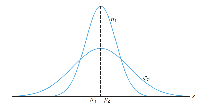
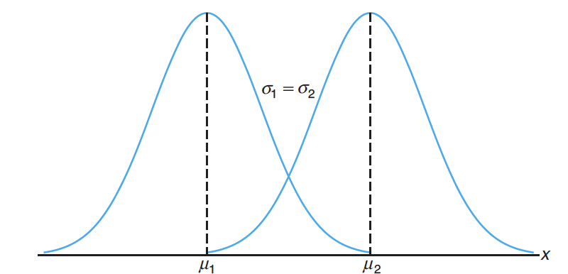
• The normal distribution (also be called Gaussian distribution) is a symmetric distribution that is centered around a mean and spreads out in both directions.
  正态分布（也被称为高斯分布）是围绕平均值和差居中出在两个方向上对称分布。

  Examples: Test scores for all ITM 514 students. 所有 ITM 514 学生的考试成绩。

• Notation: $X\sim \mathcal{N}(\mu, \sigma^2)$
  符号

  • $\mu$ is the mean of the distribution 分布的平均值
  • $\sigma^2$ is the variance of the distribution 分布的方差

• Probability Density Function pdf :

  $$f(x) = \frac{1}{\sqrt{2\pi}\sigma}e^{-\frac{(x-\mu)^2}{2\sigma^2}},\,\,\,\text{for } -\infty<x<\infty.$$

• CDF: The CDF of normal distribution doesn't have a closed form, i.e., there is no analytic answer of the integral 正态分布的 CDF 没有封闭形式，即没有积分的解析答案

$$P(X<x) = P(X \le x)=F(x) = \int_{-\infty}^x f(t)d t =\frac{1}{\sqrt{2\pi}\sigma} \int_{-\infty}^x e^{-\frac{(t-\mu)^2}{2\sigma^2}} dt$$

$$P(x_1<X<x_2) = \int_{x_1}^{x_2}f(t)dt = \frac{1}{\sqrt{2\pi}\sigma}\int_{x_1}^{x^2} e^{-\frac{(t-\mu)^2}{2\sigma^2}} dt = F(x_2) -F(x_1).$$

# Example 2

Suppose $Z$ is the standard normal random variable, i.e., $Z \sim \mathcal{N}(0, 1)$
假设 $Z$ 是标准正态随机变量

n <- 1e6 # number of sample size

x <- rnorm(n, mean = 0, sd = 1) # generate the standard normal random numbers

hist(x, probability=TRUE, col=gray(.9), main="standard normal random numbers") # histogram of the relative frequency

curve(dnorm(x, mean = 0, sd =1),add=T,col = "red") #plot the probability density function of X

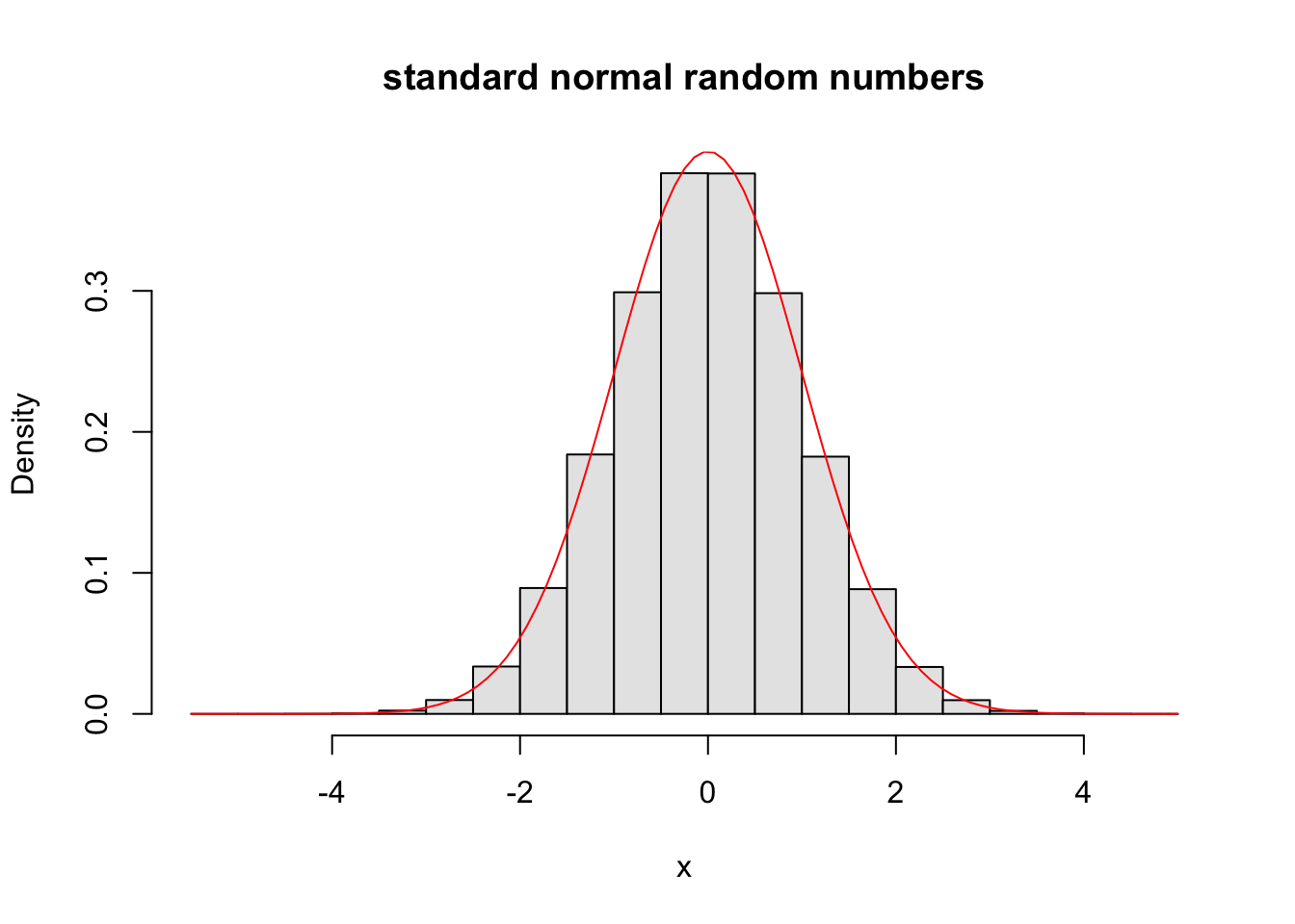
pnorm(0.5, mean =  0, sd = 1) # find the P(X <= 0.5) or P(X < 0.5)

[1] 0.6914625

qnorm(0.5, mean = 0, sd = 1) # find the median of X

[1] 0

mean(x) # find the sample mean

[1] -0.002525208

var(x)

[1] 1.002635

What's the relationship between the general normal random variable $X \sim \mathcal{N}(\mu, \sigma^2)$ and the standard normal random variable?
一般正态随机变量和标准正态随机变量有什么关系

$$Z= \frac{X-\mu}{\sigma} \sim \mathcal{N}(0,1).$$

To calculate the probability involving $X\sim \mathcal{N}(\mu,\sigma^2)$, 计算涉及的概率

# Example 3

The achievement scores from a college entrance examination are normally distributed with mean 75 and standard deviation 10. What fraction of the scores lies between 80 and 90?
高考成绩的平均分是 75，标准差是 10 的正态分布。80 到 90 之间的分数是多少？

p1<- pnorm(1.5, mean = 0, sd = 1) - pnorm(0.5, mean =  0, sd = 1) # find the P(0.5 <=Z <=1.5) 

p1 # display the answer

[1] 0.2417303

p2 <- pnorm(90, mean = 75, sd = 10) - pnorm(80, mean = 75, sd = 10) # find the P(80 <=X <=90)

p2 # display the answer

[1] 0.2417303

# Example 4

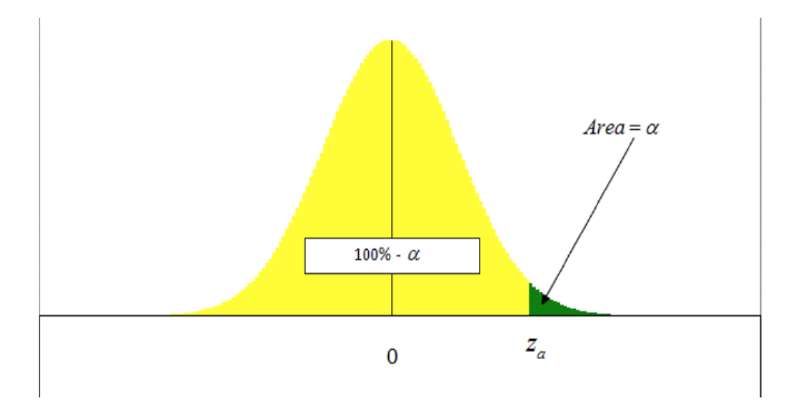
Find the value of $z_0$ such that $95\%$ of the standard normal $Z$ values lie between $-z_0$ and $z_0$; that is, $P(-z_0\leq Z\leq z_0) = .95$.
找到 $z_0$ 使 95 % 标准正常的 $Z$ 值介于 $-z_0$ 和 $z_0$ 之间

p1 <- - qnorm(0.025, mean = 0, sd = 1)  # find the P(0.5 <=Z <=1.5) 

p1 # display the answer

[1] 0.2417303

p2 <- pnorm(90, mean = 75, sd = 10) - pnorm(80, mean = 75, sd = 10) # find the P(80 <=X <=90)

p2 # display the answer

[1] 0.2417303

# In-class Exercise

Suppose $Z \sim \mathcal{N}(0,1)$,
can you find a $y>0$ such $P(-y \le Z \le y) = 0.01$?
假设 $Z \sim \mathcal{N}(0,1)$，你能找到一个 $y>0$ 且 $P(-y \le Z \le y) = 0.01$?

Critical value $z_{\alpha}$ of a standard normal distribution is the value on the measurement axis for which $\alpha$ of the are under the standard normal curve lies to the right of $z_{\alpha}$.
临界值 $z_{\alpha}$ 的标准正态分布是在测量轴上的值，对于这个 $\alpha$ 位于标准正态曲线下方的 $z_{\alpha}$。

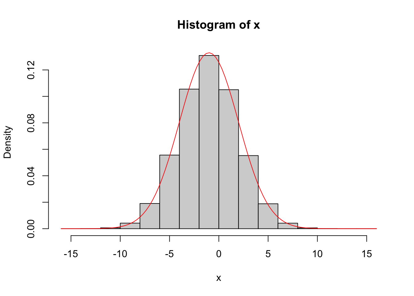
# In-class Exercise: Normal Distribution

1. Suppose $X \sim \mathcal{N}(-1,3^2)$, please generate the random numbers with sample size $n = 1e6$.
   认为 $X \sim \mathcal{N}(-1,3^2)$，请生成样本大小的随机数 $n = 1e6$.

   	#1 Create the sample
   	n <- 1e6
   	x <- rnorm(n, mean = -1, sd = 3)

2. Do a histogram for the instances you generated with the y-axis as relative frequency instead of frequency.
   使用 y 轴作为相对频率而不是频率为您生成的实例绘制直方图。

   	#2 A histogram of x
   	hist(x, probability = TRUE)
   	curve(dnorm(x, mean = -1, sd = 3), add = T, col = "red")

3. Find $P(X \le 0)$, $P(X \le 1)$, $P(X \ge 1)$, and $P( 0\le X \le 1)$.
   找 $P(X \le 0)$, $P(X \le 1)$, $P(X \ge 1)$, and $P( 0\le X \le 1)$。

   	#3 P(X <=0)
   	pnorm(0, mean = -1, sd = 3)

   [1] 0.6305587
   

   	# P(X <= 1)
   	pnorm(1, mean = -1, sd = 3)

   [1] 0.7475075
   

   	# P(X >= 1)
   	1 - pnorm(1, mean = -1, sd = 3)

   [1] 0.7475075
   

   	# P(0 <= X <=1)
   	pnorm(1, mean = -1, sd = 3) - pnorm(0, mean = -1, sd = 3)

4. Find Q1, median, Q3 of this random variable $X$. What is the expectation value and variance of $X$?
   找到这个随机变量$X$ 的 Q1、中位数、Q3，$X$ 的期望值和方差是多少 XX?

   	#4 Q1
   	qnorm(0.25, min = -1, max = 3)

   [1] -3.023469
   

   	#4 Median
   	qnorm(0.5, min = -1, max = 3)

   [1] -1
   

   	#4 Q3
   	qnorm(0.75, min = -1, max = 3)

   [1] 1.023469
   

5. Find Q1, median, Q3, mean, and variance of the sample you generated. Compare your results with the answers in Ex.4.
   找出您生成的样本的 Q1、中位数、Q3、均值和方差。将您的结果与第 4 题中的答案进行比较。

   	#4 We know the mean is -1 and variance is 9
   	#5 Q1, median, Q3 of the sample
   	quantile(x)

            0%        25%        50%        75%       100% 
   -15.773765  -3.029712  -1.010223   1.014308  14.674138
   

   	# Mean of the sample
   	mean(x)

   [1] -1.008806
   

   	#5 Variance of the sample
   	var(x)

   [1] 8.978004
   

# Conclusion

Normal distribution is the most important distribution. When we talk about the Central Limit Theorem, confidence interval, and hypothesis testing, we will come back to the normal distribution.
正态分布是最重要的分布。当我们谈论中心极限定理、置信区间和假设检验时，我们会用到正态分布。