# Neural Networks
# Artificial Neural Networks (ANN)
Researchers tried to learn from the biological neuron systems and built the ANN
研究人员试图向生物神经元系统学习,并建立了 ANN- There are many neuron units in ANN
ANN 中有许多神经元单位 - They are connected within a structure
他们是连接在一个结构 - They work as threshold switching units
他们作为阈值切换单元工作 - There are weighted interconnections among units
有加权互联单位之一 - We are able to learn and tune up these weights automatically by a training process
我们能够通过训练过程自动学习和调整这些重量
- There are many neuron units in ANN
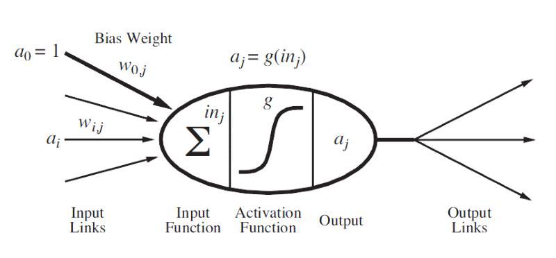
A neuron in ANN looks like this…
人工神经网络中的一个神经元看起来像这样…![]()
input signals → input function(linear) → activation function(nonlinear) → output signal
输入信号→输入函数 (线性)→激活函数 (非线性)→输出信号
# Perceptron 感知器
- First neural network learning model in the 1960’s
20 世纪 60 年代的第一个神经网络学习模型 - Simple and limited (single layer models)
简单且有限 (单层模型) - Still used in current applications (modems, etc.)
仍在当前应用中使用 (调制解调器等)。
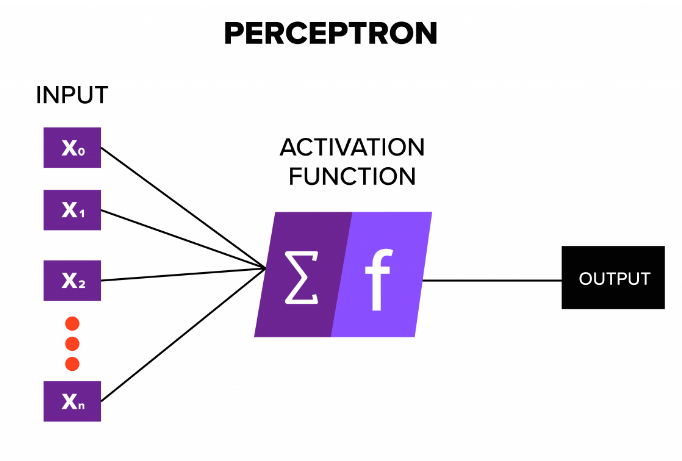
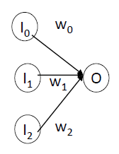
- Input 输入
- different variables with weights on edges
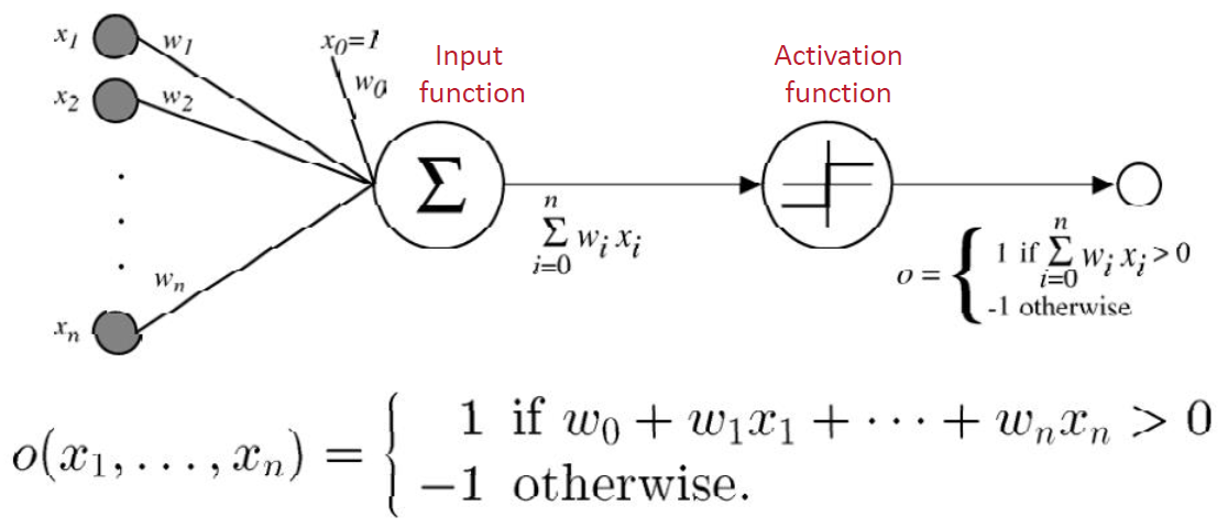
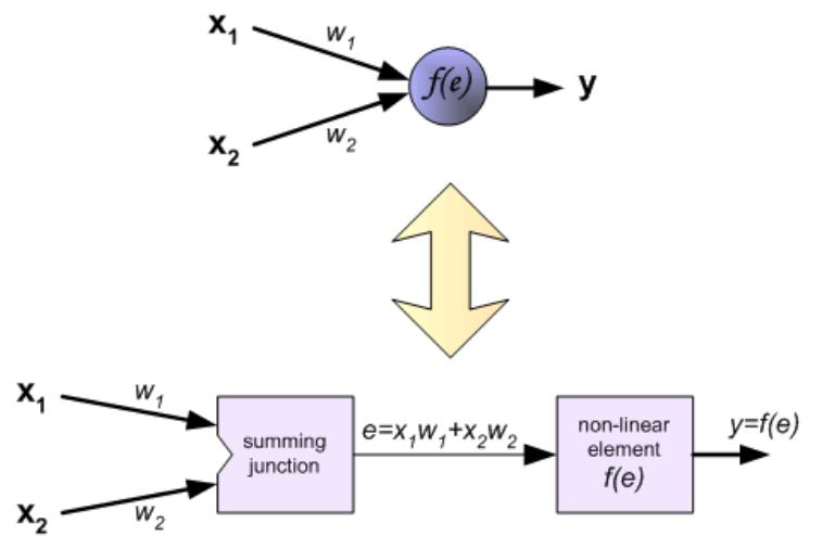
不同的 变量权重边缘 - Input function 输入函数
- it is used to aggregate the inputs, usually it is a weighted sum of its inputs
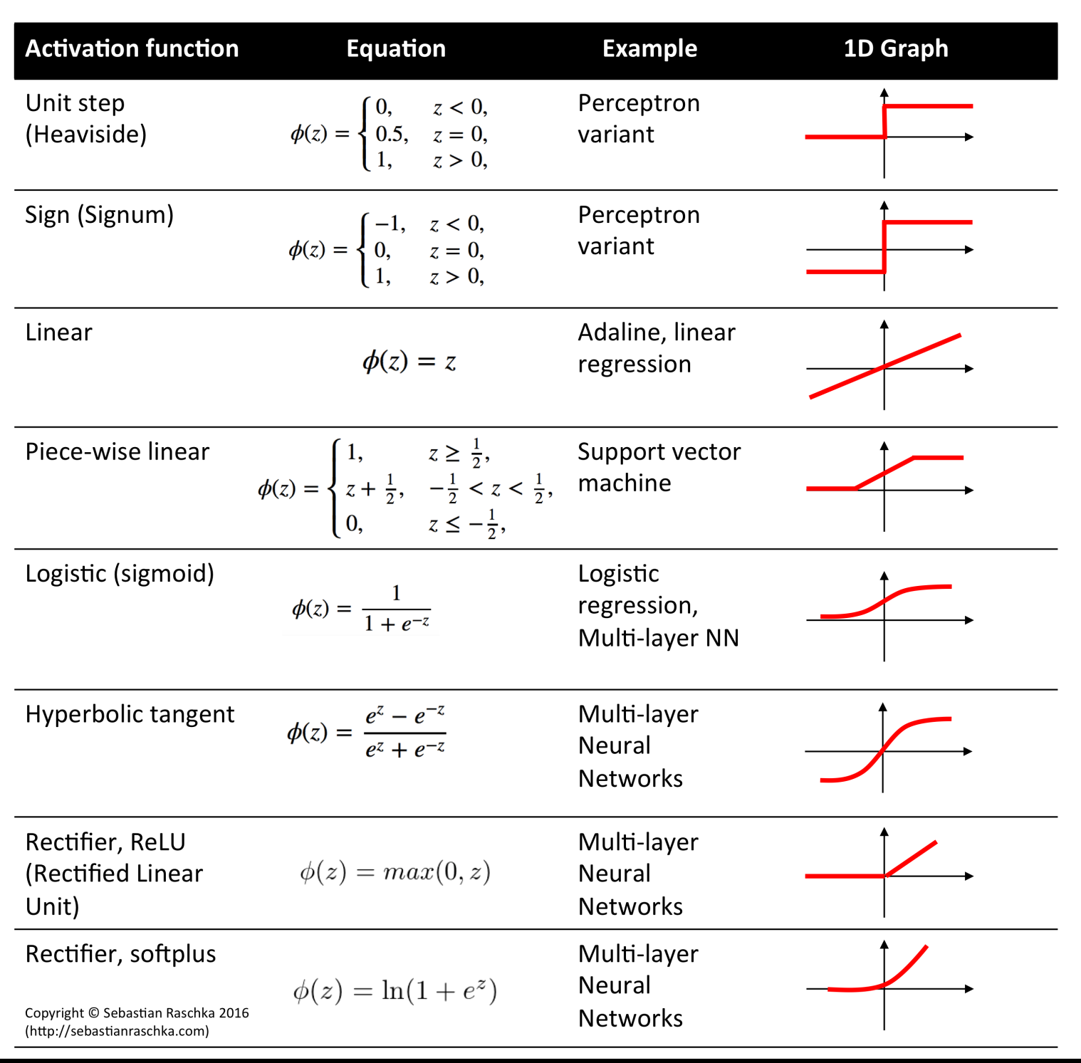
用于汇总输入,通常是其输入的加权和 - Activation function 激活函数
- It is a threshold function
是一种阈值函数 - For the purpose of binary classification
为目的的二元分类- The output is only 1 or 0
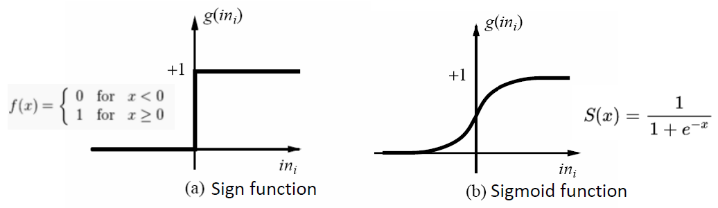
输出是只 1 或 0 - Sign function can be used as the activation function
符号函数可以用来激活功能 - Sigmoid can be used as activation function
乙状函数可用作激活函数
- The output is only 1 or 0
- It is a threshold function
- Sigmoid function 乙状函数 / S 函数
- It is popular for classification, due to being easy to be updated and learned in the training process.
由于在训练过程中易于更新和学习,是流行的分类方法。
- Neural networks canbe used for both classifications and regressions.
神经网络既可以用于分类,也可以用于回归 - It can be controlled by applying different activation functions.
可以通过施加不同的激活函数进行控制。

# Perceptron Training 感知器训练
It is the simplest ANN model
这是最简单的人工神经网络模型- We need to train the model to learn the weights, , where
我们需要训练模型来学习权重,,其中 - is the real value
是实际值 - is the output value (prediction by the model)
是输出值 (由模型预测) - is a constant value in as the learning rate
是 中的一个常数值,作为学习速率
- We need to train the model to learn the weights, , where
It is a process of iterative learning
这是一个反复学习的过程- At the beginning, give random values to
开始时,给 随机取值 - Get the output through the perceptron
通过感知器得到输出 - Update the by using the update rules
使用更新规则更新 - Stop the learning process by a stopping criterion
通过停止标准停止学习过程- Classification error is smaller than a threshold
分类误差小于阈值 - Or, maximal learning iterations have been reached
或者,已经达到最大学习迭代次数
- Classification error is smaller than a threshold
- At the beginning, give random values to
# Perceptron: Example
- Consider learning the logical OR function
考虑学习逻辑或函数
| Sample | x0 | x1 | x2 | label |
|---|---|---|---|---|
| 1 | 1 | 0 | 0 | 0 |
| 2 | 1 | 0 | 1 | 1 |
| 3 | 1 | 1 | 0 | 1 |
| 4 | 1 | 1 | 1 | 1 |
Activation function 激活函数
We’ll use a single perceptron with three inputs.
我们将使用一个有三个输入的感知器。We’ll start with all weights
0W= <0,0,0>
我们将从所有重量 0 开始
Example 1
I = <0,0,0>label = 0W = <0,0,0>- Perceptron () output =
0 - it classifies it as
0, so correct, do nothing
它将其归类为0,所以正确,什么也不做
- Perceptron () output =
Example 2
I = <1,0,1>label=1W = <0,0,0>- Perceptron () output =
0 - it classifies it as
0, while it should be1, so we add input to weightsW = <0,0,0> + <1,0,1>= <1,0,1>
它将其分类为 0,而它应该是 1,所以我们将输入添加到权重W = <0,0,0> + <1,0,1>= <1,0,1>
- Perceptron () output =
Example 3
I = <1,1,0>label = 1W = <1,0,1>- Perceptron () output =
1 - it classifies it as
1, correct, do nothingW = <1,0,1>
它将其分类为1,正确,什么都不做W = <1,0,1>
- Perceptron () output =
Example 4
I = <1,1,1>label = 1W = <1,0,1>- Perceptron () output =
1 - it classifies it as
1, correct, do nothingW = <1,0,1>
- Perceptron () output =
1st iteration is completed. 第一次迭代完成。
Repeat until no errors 重复,直到没有错误
# Limitations of Perceptron 感知器的局限性
- It is too simple, cannot learn complex and effective models
它太简单,无法学习复杂而有效的模型 - It assumes the data can be linearly separatable in the binary classification, but actually it could be non linear!
它假设数据在二元分类中可以线性分离,但实际上它可能是非线性的!- SVM, we use kernel function to map data to higher dimension
SVM,使用核函数将数据映射到更高维度 - ANN, we can add more layers!!
ANN,可以加更多的层
- SVM, we use kernel function to map data to higher dimension
# Multi layer Feed forward Networks 多层前馈网络
- Multi layer Feed forward Networks is an extension of the perceptron model. It adds hidden layers to the original perceptron.
多层前馈网络是感知器模型的扩展。它将隐藏层添加到原始感知器中。
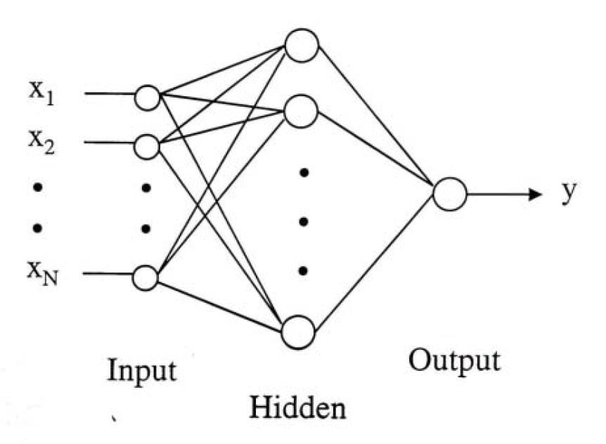
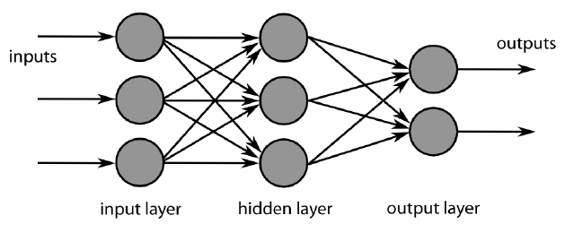
- Input layer: accepts inputs only
输入层:仅接受输入 - Hidden layers: neurons with functions
隐藏层:具有功能的神经元 - Output layer: produce outputs
输出层:产生输出
# Training Phrase
- The training phrase is a typical process of machine learning and optimization
训练阶段是机器学习和优化的典型过程 - We need to 我们需要
- Setup a learning objective as loss function
将学习目标设置为损失函数 - Use appropriate optimizer to learn the parameters
使用适当的优化器来学习参数 - It is usually a process of iterative learning
这通常是一个迭代学习的过程
- Setup a learning objective as loss function
# Loss Function 损失函数
- The loss function is defined as the amount of utility lost by predicting when the correct answer is
损失函数定义为当正确答案是 时,通过预测而损失的效用量 - Often a simplified version is used, , that is independent of
通常使用简化的版本,独立于 - Three commonly used loss functions:
三种常用的损失函数:- Absolute value loss: 绝对值损失
- Squared error loss: 平方误差损失 L_{2}\left(y, y^{\prime}\right)=\left(y-y^{\prime}\right)^
- 0/1 loss: if , else
- Let be the set of examples. Total loss
# Optimizer: Gradient Descent 优化器:梯度下降
- Gradient Descent is widely used as one of the
popular optimizers in machine learning, especially in
the ANN learning
梯度下降法是机器学习,尤其是人工神经网络学习中最常用的优化方法之一
# Optimization In Linear Regression
- How to apply gradient descent to minimize the cost function for regression
如何应用梯度下降来最小化回归的成本函数- a closer look at the cost function
仔细看看成本函数 - applying gradient descent to find the minimum of the cost function
应用梯度下降来寻找成本函数的最小值
- a closer look at the cost function
# a closer look at the cost function
Hypothesis: 假设
Parameters: 参数
Cost Function: 成本函数
Sum of squared errors 误差平方和Goal:
Optimization
- There are at least two optimization methods
至少有两种优化方法- Least square optimization
最小平方优化 - Optimization based on gradient descent
基于梯度下降的优化
- Least square optimization
- There are at least two optimization methods
Least Square Optimization 最小平方优化
- Find the optimal point 找到最佳点
, is the objective function with $\theta_{1}, \theta_{2}, \theta_{3}, \ldots $ - , assume have variables
- Therefore, you will have functions to be solved
因此,将有 个函数需要求解 - Drawback: it is complicated if you have many variables
缺点:如果有许多 变量,这就复杂了
- Find the optimal point 找到最佳点
# applying gradient descent to find the minimum of the cost function
Have some function
Want
Gradient descent algorithm outline: 梯度下降算法概述:
- Start with some ;
- Keep changing to reduce until we hopefully end up at a minimum
# Backpropagation Training 反向传播训练
- There are several network structure in neural networks, such as feed forward neural networks and the recurrent neural networks
神经网络有几种网络结构,如前馈神经网络和递归神经网络 - Multi layer Feed forward Networks used a forward procedure for predictions.
多层前馈网络使用前向程序进行预测。
But it was trained by using a Backward propagation approach
但它是用反向传播方法训练的 - These ANNs are also called BP (Backpropagation) Neural Networks
这些人工神经网络也被称为 BP (反向传播) 神经网络
# ANN needs a process of weight training
- A set of examples, each with input vector and output vector
一组例子,每个例子都有输入向量 和输出向量。 - Squared error loss: , where is the -th output of the neural net
- The weights are adjusted as follows:
- How can we compute the gradient efficiently given an arbitrary network structure?
- Answer: backpropagation algorithm
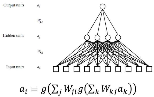
# Forward vs Backward in ANN
- Forward phase:
- Propagate inputs forward to compute the output of each unit
- Output at unit : where .
- Backward phase:
- Propagate errors backward
- For an output unit :
- For an hidden unit : .


# Forward in ANN:


# Backward in ANN


# Neural Networks and Deep Learning
To make ANN more powerful, there are two solutions
为了使 ANN 更加强大,有两种解决方案- Add more neurons in the hidden layer
在隐藏层中添加更多的神经元 - Add more hidden layers
添加更多隐藏层
- Add more neurons in the hidden layer
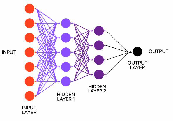
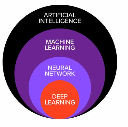
Deep Learning Deep Learning
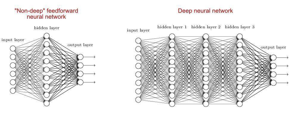
- Traditional ANN only has 3 layers. Deep learning utilizes neural networks with multiple layers
传统的人工神经网络只有 3 层。深度学习利用多层神经网络 - Deep learning have more structures for neural networks, such as ANN, Convolutional Neural Networks (CNN), Recurrent Neural Networks (RNN), and so forth
深度学习有更多的神经网络结构,如 ANN、卷积神经网络 (CNN)、递归神经网络 (RNN) 等等 - Deep learning is not related to neural networks only. It also correlates with computing, such as GPU
深度学习不仅仅与神经网络相关。它还与计算相关,如 GPU
- Traditional ANN only has 3 layers. Deep learning utilizes neural networks with multiple layers
ANN vs Deep Learning
# Ensembles of Classifiers 分类器集合
- Basic idea is to learn a set of classifiers (experts) and to allow them to vote.
基本思想是学习一组分类器 (专家) 并允许他们投票。 - Advantage: improvement in predictive accuracy.
优点:预测精度提高。 - Disadvantage: it is difficult to understand an ensemble of classifiers.
缺点:很难理解分类器的集成。
# Ensemble Methods 集成方法
# Bagging
Process in bagging 装袋过程
- Sample several training sets of size (instead of just having one training set of size )
采样几个大小为 的训练集 (而不是只有一个大小为 的训练集) - Build a classifier for each training set
为每个训练集构建一个分类器 - Combine the classifier’s predictions by voting or averaging
通过投票或平均来组合分类器的预测
- Sample several training sets of size (instead of just having one training set of size )
Bagging classifiers
- Classifier generation
Let n be the size of the training set. For each of t iterations: Sample n instances with replacement from the training set. Apply the learning algorithm to the sample. Store the resulting classifier.- classification
For each of the t classifiers:
    Predict class of instance using classifier.
Return class that was predicted most often.
Voting and Averaging 投票和平均
- Voting is used for classifications, and averaging is used for regressions
投票用于分类,平均用于回归 - Voting: Hard and Soft voting
投票:硬投票和软投票
- Voting is used for classifications, and averaging is used for regressions
Hard voting
Predictions:Classifier 1 predicts class A
Classifier 2 predicts class B
Classifier 3 predicts class B2/3classifiers predict class B, so class B is the ensemble decision.Soft voting
Predictions (identical to the earlier example, but now in terms of probabilities.Shown only for class A here because the problem is binary):Classifier 1 predicts class A with probability 99%
Classifier 2 predicts class A with probability 49%
Classifier 3 predicts class A with probability 49%
The average probability of belonging to class A across the classifiers is(99+49+49)/3 = 65.67%.
Therefore, class A is the ensemble decision.Why does bagging work?
- Bagging reduces variance by voting / averaging, thus reducing the overall expected error
- In the case of classification there are pathological situations where the overall error might increase
- Usually, the more classifiers the better
- Bagging reduces variance by voting / averaging, thus reducing the overall expected error
# Boosting
Also uses voting/averaging but models are weighted according to their performance
Iterative procedure new models are influenced by performance of previously built ones
- New model is encouraged to become expert for instances classified incorrectly by earlier models
- Assign more weights to the misclassified instances to improve the classification iteratively
There are several variants of this algorithm
AdaBoost.M1
- classifier generation
Assign equal weight to each training instance. For each of t iterations: Learn a classifier from weighted dataset. Compute error e of classifier on weighted dataset. If e equal to zero, or e greater or equal to 0.5: Terminate classifier generation. For each instance in dataset: If instance classified correctly by classifier: Multiply weight of instance by e / (1 - e) Normalize weight of all instances.- classification
Assign weight of zero to all classes.
For each of the t classifiers:
    Add -log(e / (1 - e)) to weight of class predicted by the classifier.
Return class with highest weight.
# Random Forest
Random forest is a bagging method which uses decision trees as the classifiers
The workflow in the random forest is the same as the ones in bagging
In bagging, we can use any classifiers In random forest, we use decision trees
Classifier generation
Let n be the size of the training set.
For each of t iterations:
    (1) Sample n instances with replacement from the training set
    (2) Learn a decision tree s.t. the variable for any new node is the best variable among m randomly selected variables.
    (3) Store the resulting decision tree.
Classification
For each of the t decision trees:
    Predict class of instance.
Return class that was predicted most often.
# Semi-Supervised Classification 半监督分类
Classifications require labeled data
Data labeling is a complicated and expensive process. It is not guaranteed that we have enough and high qualified labels
Labels may be hard to get
- Human labeling is slow and boring
- It may require expert knowledge
- It may require special or expensive devices
Goal:
Using both labeled and unlabeled data to build better classifiers (than using labeled data alone).Notation:
- input , label
- classifier f: \mathcal{X} \mapsto \mathcal
- labeled data
- unlabeled data
- usually
# Solutions: Self-training
- Algorithm: Self-training
- Pick your favorite classification method. Train a classifier from .
- Use to classify all unlabeled items .
- Pick with the highest confidence, add to labeled data.
- Repeat.
The simplest semi-supervised learning method.
Pros
- Simple
- Applies to almost all existing classifiers
Cons
- Mistakes reinforce themselves. Heuristics against pitfalls
- 'Un-label' a training point if its classification confidence drops below a threshold
- Randomly perturb learning parameters
# Solutions: Co-training
Your data can be split into different views
The view can be defined by different set of the features
Each item is represented by two kinds of features
- = image features
- = web page text
- This is a natural feature split (or multiple views)
Co-training idea:
- Train an image classifier and a text classifier
- The two classifiers teach each other
Algorithm: Co-training
- Train two classifiers: from from
- Classify with and separately.
- Add 's -most-confident to 's labeled data.
- Add 's -most-confident to 's labeled data.
- Repeat.
Pros
- Simple. Applies to almost all existing classifiers
- Less sensitive to mistakes
Cons
- Feature split may not exist
- Models using BOTH features should do better
# Multi-Label Classifications

Binary classification: Is this a picture of the sea?
Multi-class classification: What is this a picture of?
Multi-label classification: Which labels are relevant to this picture?
i.e., multiple labels per instance instead of a single label!
# Applications

.")

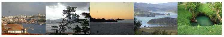
Images are labelled to indicate
- multiple concepts
- multiple objects
- multiple people
e.g., Scene data with concept labels
Labelling music/tracks with genres / voices, concepts, etc.
- e.g., Music dataset, audio tracks labelled with different moods, among:
- amazed-surprised,
- happy-pleased,
- relaxing-calm,
- quiet-still,
- sad-lonely,
- angry-aggressive
- e.g., Music dataset, audio tracks labelled with different moods, among:
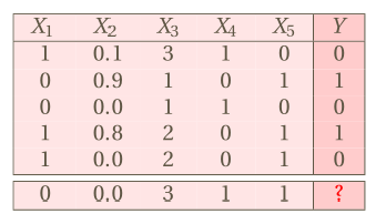
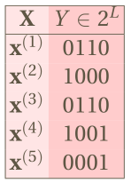
# Example
Difference in data sets
Table: Single-label .
![]()
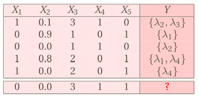
Table: Multi-label
![]()
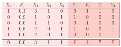
We usually convert labels to binary labels
![]()
# Solutions
# Transformation Based Methods
Transform the task to binary/multi-class classifications
# Binary Relevance
- If there are labels, we have binary classifications
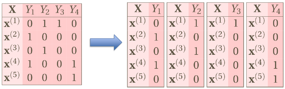
- Drawback: it ignores the label depenence
# Classifier Chains
- Classifier Chains build the model in a chain by taking label correlations into consideration
- It uses the feature to perform binary classification on 1st label, the prediction on 1st label will be reused as the features into the 2nd step to predict the 2nd label
- Repeat the process above until all of the labels are predicted
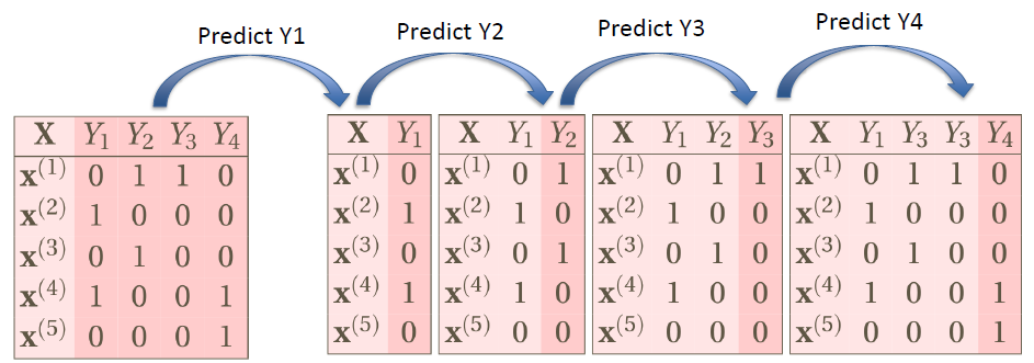
Use previous prediction results as new features
Drawbacks in Classifier Chains
- Difficult to define the sequence in the chain, though there are some methods (e.g., info gain)
- If the previous predictions are incorrect, the following predictions may not be right too.
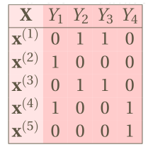
# Label Powerset
Each subset of the label set will be a single label
Assign binary classification or multi-class classification to them
Find a way to aggregate the results
- Transform dataset
![]()
...into a multi-class problem, taking possible values:![]()
- ...and train any off-the-shelf multi-class classifier
- Transform dataset
Drawbacks in Label Powerset
标签权力集的缺点- Too many subsets if there are several labels
如果有多个标签,则有太多的子集 - Highly possible to have imbalance issue
极有可能出现不平衡的问题 - Overfitting: how to predict new values/labels?
过度拟合:如何预测新值 / 标签?
- Too many subsets if there are several labels
# Adaptation Based Methods 基于适应性的方法
Develop new algorithms to solve the problem
开发新的算法来解决这个问题
# Algorithm adaptation techniques
- MLkNN.For each test instance:
- Retrieve the top-k nearest neighbors to each instance
- Compute the frequency of occurrence of each label
- Assign a probability to each label and select the labels by using a probability cut-off value
# Evaluation of multilabel learning
Notes
- Both transformation and adaptation methods are the methods to solve MLC problem
- They are not classification algorithms
- For each method, you can use any traditional binary/multi-class classification algorithms to produce the predictions
- There are multiple labels in the MLC problem
- Traditional evaluation metrics in the classification may not work for MLC
- We need to develop new evaluation metrics
# Hamming Loss
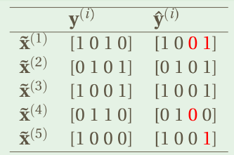
Consider the misclassification in each bit
N = # of labels
L = # of data rows
# 0/1 Loss
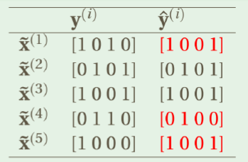
Consider the misclassification in the whole label set
# Other Metrics
- JACCARD INDEX
- often called multi-label ACCURACY
- RANK LOSS
- average fraction of pairs not correctly ordered
- ONE ERROR
- if top ranked label is not in set of true labels
- COVERAGE
- average "depth" to cover all true labels
- LOG LOSS
- i.e., cross entropy
- PRECISION
- predicted positive labels that are relevant
- RECALL
- relevant labels which were predicted
- PRECISION VS. RECALL curves
- F-MEASURE
- micro-averaged ('global' view)
- macro-averaged by label (ordinary averaging of a binary measure, changes in infrequent labels have a big impact)
- macro-averaged by example (one example at a time, average across examples)
# Tools
- Mulan
- Java Based
- Reuse Weka library
- No UI
- http://mulan.sourceforge.net/
- Meka
- Similar to Weka
- Java Based
- With UI
- http://meka.sourceforge.net/
# Classification: Summary
We learned different algorithms
- No learning process: KNN and Naïve Bayes
- Learning based: Logistic regression, Decision tree, SVM, Neural Networks
- Ensemble methods: bagging, boosting, RandomForest
For each algorithm 对于每一种算法
- Understand how it works
了解它是如何工作的 - Know the requirements on the data; Know how to prepare a preprocessed data set
知道对数据的要求;知道如何准备一个预处理的数据集 - Know what are the parameters to be tuned up
知道哪些是需要调整的参数 - Know the solutions for overfittings
知道超配的解决方案 - Which algorithm is the best?
哪种算法是最好的?- It varies from data to data
不同的数据会有不同的结果 - We need to tune parameters to tune up the model
我们需要调整参数来调优模型 - We need to compare different classification models
我们需要比较不同的分类模型
- It varies from data to data
- General issue: imbalance in labels
一般问题:标签的不平衡性
- Understand how it works